Load Cell Basics and interfacing load cell with arduino using HX711 amplifier

A load cell is a transducer which converts force into an electrical output. They are commonly used in everyday life- measuring balance in regular grocery shop.  The working of a load cell differs based on its type- hydraulic load cell, pneumatic load cell, and strain gauge load cells.

The strain gauge type load cell most popular. It is comprised of one or more strain gauges bonded to the surface of a metal structure with known elastic properties. The commonly used metal is Aluminum or SS. This metal structure will stretch and compress with applied force. Strain gauges are electrical conductor firmly attached to a film in definite pattern. The strain gauges bonded to this structure measure the strain, translating applied force into electrical resistance changes. These strain gauges are arranged in what is called a bridge circuit, or more precisely a Wheatstone bridge circuit as shown in diagram below. The force on the load cell is measured by voltage change in the strain gauge due to deformation. Strain gauge load cells offer accuracies from within 0.03% to 0.25% of full scale.

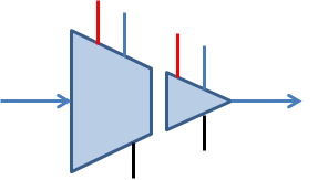
Modern load cells have 4 strain gauges installed within so as to increase accuracy. The arrangement is as shown in Figure above. Two gauges (R1 and R4) are under tension and two (R2 and R3) are in compression. When the cylindrical shaft is subjected to a force, it tends to change in dimension. Due to this resistance of strain gauges change.

When there is no load on the load cell, the resistances of each strain gauge will be the same. Under the application of force, the resistance of the strain gauge varies, causing a change in output voltage. The change in output voltage is measured and converted into readable value.

Types of load cells

There are different types of load cells for different applications. Commonly used ones include:

• Single point load cells: a load cell is located under a platform that is loaded with a weight from above.
• Bending beam load cells: several load cells are positioned under a steel structure and are loaded with a weight from above.
• Compressive force load cells: several high-capacity load cells are positioned under a steel structure that is loaded with a weight from above.
• Tensile load cells: a weight is suspended from one or more load cells.

Installation

The performance of a load cell depends on many factors. Central among these is proper installation and alignment. As such, it is important to follow the manufacturer’s recommendations carefully in order to get the best results from your device and to ensure safe and long-lasting use. These recommendations often include information on proper mounting and alignment of your load cell, appropriate fixing and fastener choice, the use of accessory mounting hardware, electronic adjuncts and calibration procedures

Four strain gauges are positioned on the load cells below at the point where the greatest deformation occurs when force is applied. The arrow is pointing the direction of force application.

Environmental effects on load cells

One special feature of load cells is that the environment in which they are used plays a decisive role – in a number of ways.

Ambient temperature

Every material changes with temperature, expanding in response to heat and contracting in response to cold. And the same applies to load cells and their strain gauges. This also changes the electrical resistance of the conductor. Yet load cells must measure the correct weight everywhere, regardless of the ambient temperature. To achieve this, a temperature compensation mechanism has to be built in load cell.

Load cell interfacing with Arduino

With the availability of low cost development board like Arduino, it has become easier to understand load cell even at home. For interfacing a load cell with we will use an amplifier board HX711 which provides 24-bit data equivalent to load. This board is specially designed for amplifying the signals from load cells and transferring the data to Arduino. The load cells plug into this board, and this board tells the Arduino what the load cells measure.

We will use a 20kg load cell for demonstration purpose. The load cells are available with 4-wires as well as 6-wires configuration. Figure below shows 4-wire load cell which we will use to interface with HX-711 amplifier.

The wiring between load cell and HX711 amplifier module is tabulated below.

Load cell wire	HX-711
Red	E+
Black	E-
White	A-
Green	A+

The connections between Arduino and HX711 module is tabulated below.

Arduino	HX-711
5 V	Vcc
2	SCK
3	DT
GND	GND

It is required to download HX711 library from Arduino IDE library manager.

Arduino code is

#include "HX711.h"

 

// HX711 circuit wiring

const int LOADCELL_DOUT_PIN = 2;

const int LOADCELL_SCK_PIN = 3;

 

HX711 scale;

 

void setup() {

  Serial.begin(57600);

  scale.begin(LOADCELL_DOUT_PIN, LOADCELL_SCK_PIN);

}

 

void loop() {

 

  if (scale.is_ready()) {

    long reading = scale.read();

    Serial.print("HX711 reading: ");

    Serial.println(reading);

  } else {

    Serial.println("HX711 not found.");

  }

 

  delay(1000);

 

}

Signal Isolation Techniques- analog and digital signal isolation

There are many applications where it is required for one system to have no direct electrical connection with the other system. Such isolation is called Galvanic isolation. This is necessary to avoid the possibility of dangerous voltages or currents from one half of the system causing damage to the other, or to break ground loop. Such a system is said to be "isolated", and the arrangement that passes a signal without galvanic connections is known as an isolation barrier.

The protection of an isolation barrier works in both directions. The common applications where a sensor may accidentally encounter high voltages and the system it is driving must be protected.

An isolation amplifier provides dc isolation between input and output. It is used for the protection of human life or sensitive equipment in those applications where high-voltage transients or power leakage are possible. An isolation amplifier consists of two electrically isolated stages. The input stage and the output stage are separated from each other by an isolation barrier so that a signal must be processed in order to be coupled across the isolation barrier.

Complete isolation of two electrical system include- signal isolation, power isolation.

Application

·         To protect human operators,

·         To protect low-voltage circuitry from high voltages,

·         To improve noise immunity,

·         To reject common mode voltage,

·         To eliminate ground loop,

·         To handle ground potential differences between communicating subsystems.

Types of signal isolation

1.      Optical Isolation

2.      Transformer/ magnetic/ inductive isolation

3.      Capacitive isolation

Some isolation amplifiers use optical coupling or transformer coupling to provide isolation between the stages. However, many modern isolation amplifiers use capacitive coupling for isolation. Each stage has separate supply voltages and grounds so that there are no common electrical paths between them.

The most common isolation amplifiers use transformers, which exploit magnetic fields, and another common type uses small high voltage capacitors, exploiting electric fields.

Optical isolation

Optoisolators, which consist of an LED and a photodiode/ phototransistor, provide isolation by using light. Optical isolators are fast and cheap, and can be made with very high voltage ratings (4 -7 kV is one of the more common ratings), but they have poor analog linearity, and are not usually suitable for direct coupling of precision analog signals.

Analog optocoupler

The analog optocouplers can be used to isolate analog signals in a wide variety of applications that require good stability, linearity, bandwidth and low cost. HCNR200/201 is popular analog optocoupler. Their circuit schematic is as shown below.

 

The figure below shows  the working circuit of analog voltage isolator using HCNR200.

The ratio of R3/R1 can be selected to provide amplification to the input signal. The ground for input stage (left side) must be separated from ground for output stage (right side). Separate set of power supplies or isolated DC-to-DC converters can be used for this purpose.

Digital optocoupler

The classic digital isolator is the LED/transistor opto-isolator. It can provide isolation upto 10kV or more. Higher speed couplers incorporate an active receiver circuit with a logic-level output.

Transformer isolation

Electromagnetic isolators such as small signal transformers are useful for AC signal isolation. Transformers like audio transformer have their primary and secondary sides isolated which can be used for different audio signal isolation. Another most common use is in network hardware or Ethernet section. Pulse transformers are used to isolate the external wiring with internal hardware. Even telephone lines are used transformer based signal isolators. But, as transformers are isolated by electromagnetically, it only works with AC.

Transformers are capable of analog accuracy of 12-16 bits and bandwidths up to several hundred kHz, but their maximum voltage rating rarely exceeds 10 kV, and is often much lower.

Capacitive isolation

The least popular method for isolating circuits is by using capacitors. Due to poor efficiency and dangerous failure outcomes this is no longer preferred. Capacitors block DC and allow passing a high-frequency AC signal. Due to this property, the capacitor is used as isolators in designs where DC currents of two circuits need to be blocked but still allowing high frequency data transmission.

Capacitive-coupled isolation amplifiers have lower accuracy, perhaps 12-bits maximum, lower bandwidth, and lower voltage ratings—but they are low cost.

Characteristics

·         Linearity- It is desirable that the relation between input and output signal is linear. Modern isolation techniques make it possible to achieve linearity as low as 0.01%.

·         Isolation voltage- It is the maximum voltage on side that can be withstand by the isolation barrier between two stages. Beyond isolation voltage, the barrier breaks down.

·         Bandwidth- It is the frequency range of input signal that can be coupled at the output without significant attenuation.

·         Transfer gain- Ratio of output signal to input signal.

LM35 temperature sensor signal processing and LabVIEW interfacing

Semiconductor temperature sensors offer high accuracy and high linearity over an operating range of about –55°C to +150°C. The output is scaled to give sensitivity of 10mV/°C. They are also useful in cold-junction compensation circuits for wide temperature range thermocouples.

All semiconductor temperature sensors make use of the relationship between a bipolar junction transistor's (BJT) base-emitter voltage to its collector current:

where k is Boltzmann's constant, T is the absolute temperature, q is the charge of an electron, and Is is a current related to the geometry and the temperature of the transistors.

The LM35/36/37 are voltage output temperature sensors with a 10mV/°C (LM35/36) or 20mV/°C (LM37) scale factor. Supply current is below 50µA, providing very low self-heating (less than 0.1°C in still air). The LM35 provides a 250mV output at +25°C and reads temperature from +10°C to +125°C. LM35 have an output scale factor of +10mV/°C.

LT1167 Single Resistor Gain Programmable, Precision Instrumentation Amplifier

As the output from LM35 is very low (typically 300 mV at 30°C), it is susceptible to distortion due to noise. The signal is amplified using an amplifier to a suitable level so as to utilize the full input range of ADC of Arduino. It improves the measurement sensitivity.

We are using LT1167 precision In-amp from Linear Technologies (now Analog Devices).

Supply voltage: ±15 VDC

Setup and connection

REF pin (5) is to be connected to Ground.

We have selected Rg=8.2kΩ. So the gain is 7.02.

The amplified output is fed to analog input channel of an Arduino UNO board. The data is read on LabVIEW using Makerhub example program for Single Channel AI read. I tweaked the program to display temperature in degree C.

Working with PIR sensor on Arduino

PIR Sensor

PIR Sensor stands for Pyroelectric (passive) InfraRed sensor, which allows us to detect human or object movement within a certain range. They are small, low-cost, low-power, easy to use and long lasting. PIR sensors are adopted in myriads of projects as they are easy to use with popular hardwares such as Arduino and raspberry pi. PIR sensors are commonly used in security alarms and automatic lighting applications.

Working of PIR sensor

PIRs are basically made of a pyroelectric sensor, which can detect levels of infrared radiation and convert IR energy to electrical signal. All bodies with temperature above absolute zero (0 K) emit infra-red radiation. The higher the temperature, the more radiation is emitted. The sensor in a motion detector is actually split in two halves. When a body moves, the sensor detects change in IR levels. The two halves are connected in a way so that they cancel each other out. If one half sees more or less IR radiation than the other, the output will swing high or low.

If the human infrared radiation is directly irradiated on the detector, it will output a signal. The signal strength depends on distance from body.  Farther the distance, lesser is the irradiation on sensor and lesser is the sensitivity. In order to lengthen the detection distance of the detector, an optical system is added to focus the infrared radiation, usually using a plastic optical reflection system or a Fresnel lens made of plastic as a focusing system for infrared radiation.

In the detection area, the infrared radiation energy of the human body through the clothing is received by the lens of the detector and focused on the pyroelectric sensor. The detector can sense the human body within a field of view . The pyroelectric sensor sees the moving human body till it is within field of view and then does not see it beyond that. The infrared radiation constantly changes the temperature of the pyroelectric material so that it outputs a corresponding signal, which is the alarm signal.

Most PIR sensors have a 3-pin connection at the side or bottom. One pin will be ground, another will be signal and the last pin will be power. Power is usually up to 5V. Interfacing PIR with Arduino is very easy and simple. The PIR acts as a digital output so all you need to do read the output state as HIGH or LOW. The motion can be detected by checking for a high signal on a single I/O pin. Once the sensor warms up the output will remain low until there is motion, at which time the output will swing high for a couple of seconds, then return low. If motion continues the output will cycle in this manner until the sensors line of sight of still again. The PIR sensor needs a warm-up time with a specific end goal to capacity fittingly. The settling is adjustable from 10-60 seconds.

The Range of PIR Sensor

Indoor passive infrared: 25 cm to 20 m.

Indoor curtain type: 25 cm to 20 m.

Outdoor passive infrared: 10 meters to 150 meters.

Outdoor passive infrared curtain detector: 10 meters to 150 meters

Interfacing with Arduino

There are three pins in the PIR sensor- Vcc, OUTPUT, GND. We connect Vcc pin to +5V terminal of Arduino, GND to Ground pin and OUTPUT to any digital input pin of arduino.

Arduino code

/*

  DigitalReadSerial

  Reads a digital input on pin 8, prints the result to the Serial Monitor

// digital pin 12 has a LED attached to it.

int PIR_OUT = 8;

int LED = 12;

// the setup routine runs once when you press reset:

void setup() {

  // initialize serial communication at 9600 bits per second:

  Serial.begin(9600);

  // make the pushbutton's pin an input:

  pinMode(PIR_OUT, INPUT);

  pinMode(LED, INPUT);

}

// the loop routine runs over and over again forever:

void loop() {

  // read the input pin:

  int State = digitalRead(PIR_OUT);

  // print out the state of the button:

  Serial.println(State);

  digitalWrite(LED, State);

  delay(200);        // delay in between reads for stability

}

Analog voltage multiplier and voltage divider circuit

Analog Voltage Multiplier

The output V_o1 of first log amplifier is given as:

The output V_o2 of second log amplifier is given as:

The output stage is an adder circuit. Its output is given as:

where

We can see that the output Vo is related to product of two inputs. This circuit acts as “ANALOG VOLTAGE MULTIPLIER”. Such circuits find their applications in Power monitoring.

Log and Antilog Amplifier

Log and antilog amplifiers are used in applications that require compression of analog input data, linearization of transducers that have exponential outputs, and analog multiplication and division. A logarithmic (log) amplifier produces an output that is proportional to the logarithm of the input, and an antilogarithmic (antilog) amplifier takes the antilog or inverse log of the input.

Logarithmic Amplifier

When you place a diode in the feedback loop of an opamp circuit, as shown in Figure below, it acts as a log amplifier. The output is limited to a maximum value of approximately -0.7V because the diode’s logarithmic characteristic is restricted to voltages below 0.7 V.

Since the forward current trough a diode is given by,

As ID = IF,

The term kT/q is a constant equal to approximately 25 mV at 25°C. Therefore, the output voltage can be expressed as

From last equation, you can see that the output voltage is the negative of a logarithmic function of the input voltage. The value of the output is controlled by the value of the input voltage and the value of the resistor R. The other factor, I_o is a constant for a given diode.

Anti-Logarithmic Amplifier

An antilog amplifier is formed by connecting a diode at the input side. The output voltage is determined by the current through the feedback resistor.

As ID = IF and Vin = VD

Control Valve Characteristics

The valve’s flow characteristic is the relationship of the change in the valve’s opening to the change in flow through the valve. In general, the flow through a control valve for a specific fluid at a given temperature can be expressed as

where  Q= volumetric flow rate

            X= valve stem position
            P₀= upstream pressure
            P₁= downstream pressure

Lets us express the following quantities:

where  Q = flow rate
Q_max = maximum flow rate
X = stem position
X_max = maximum stem position

The types of valve characteristics can be defined in terms of the sensitivity of the valve, which is the fractional change in flow to the fractional change in stem position for fixed upstream and downstream pressures. Mathematically control valve sensitivity may be expressed as:

Depending on value of can be decreasing, linear or increasing the valve characteristics can be quick opening, linear, and equal percentage respectively.

The quick-opening valve is predominantly used for on/off control applications. A relatively small movement of the valve stem causes the maximum possible flow rate through the valve. For example, a quick-opening valve may allow 85 percent of the maximum flow rate with only 25 percent stem travel.

The linear valve has a flow rate that varies linearly with the position of the stem. This relationship can be expressed as follows:

where ‘α’ is constant.

The equal percentage valve is manufactured so that a given percentage changes in the stem position produces the same percentage change in flow. Generally, this type of valve does not shut off the flow completely in its limit of travel. For an equal-percentage valve, the defining equation is

Here ‘β’ is constant.

Here q₀ is the flow at x=0.

At x = 1, q=1,

Q_min represents the minimum flow when the stem is at one limit of its travel. At the fully open position, the control valve allows a maximum flow rate, Qmin. So we define a term called Rangeability (R) as the ratio of maximum flow (Qmax) to minimum flow (Qmin):

The curve in Figure 4 shows a typical equal percentage curve that depends on the rangeability for its exact form. The curve shows that increase in flow rate for a given change in valve opening depends on the extent to which the valve is already open. This curve is typically exponential in form and is represented by: