Control Valve Characteristics

The valve’s flow characteristic is the relationship of the change in the valve’s opening to the change in flow through the valve. In general, the flow through a control valve for a specific fluid at a given temperature can be expressed as

where  Q= volumetric flow rate

            X= valve stem position
            P₀= upstream pressure
            P₁= downstream pressure

Lets us express the following quantities:

where  Q = flow rate
Q_max = maximum flow rate
X = stem position
X_max = maximum stem position

The types of valve characteristics can be defined in terms of the sensitivity of the valve, which is the fractional change in flow to the fractional change in stem position for fixed upstream and downstream pressures. Mathematically control valve sensitivity may be expressed as:

Depending on value of can be decreasing, linear or increasing the valve characteristics can be quick opening, linear, and equal percentage respectively.

The quick-opening valve is predominantly used for on/off control applications. A relatively small movement of the valve stem causes the maximum possible flow rate through the valve. For example, a quick-opening valve may allow 85 percent of the maximum flow rate with only 25 percent stem travel.

The linear valve has a flow rate that varies linearly with the position of the stem. This relationship can be expressed as follows:

where ‘α’ is constant.

The equal percentage valve is manufactured so that a given percentage changes in the stem position produces the same percentage change in flow. Generally, this type of valve does not shut off the flow completely in its limit of travel. For an equal-percentage valve, the defining equation is

Here ‘β’ is constant.

Here q₀ is the flow at x=0.

At x = 1, q=1,

Q_min represents the minimum flow when the stem is at one limit of its travel. At the fully open position, the control valve allows a maximum flow rate, Qmin. So we define a term called Rangeability (R) as the ratio of maximum flow (Qmax) to minimum flow (Qmin):

The curve in Figure 4 shows a typical equal percentage curve that depends on the rangeability for its exact form. The curve shows that increase in flow rate for a given change in valve opening depends on the extent to which the valve is already open. This curve is typically exponential in form and is represented by:

Pressure measurement - Boudan Tube Gauge

Bourdon tube is a type of flexible mechanical pressure measuring device. The pressure changes the shape of the measuring element in proportion to the applied pressure. A metallic flexible pressure measuring element can only be deformed within a limited range due to the considerable material stresses involved. Pressure gages using this principle measure pressures above atmospheric to several thousand psi. They are available in C-shape, Helical and spiral shapes.

C-Bourdon Pressure Gauge

The C-type Bourdon tube is made by folding a tube to form segment of a circle, usually an arc of 250°. The process medium whose pressure is to be measured is connected to the fixed end of the tube, while the other end is sealed. Because of pressure difference between inner tube wall and outer tube wall, the Bourdon tube tends to straighten. The sealed tip end moves in non-linear trajectory. By means of mechanical sector and pinion arrangement, this non-linear motion of tip is amplified and converted to linear motion of pointer.

Commonly used material for making Bourdon Tube

1. Phosphor Bronze
2.  Beryllium copper
3. SS 316M
4. Monel
5. Inconel

Direct measuring C-Bourdon tubes can measure in the span from 0-15 PSI to 0-20000 PSI. Not suitable for very low pressure. The accuracy is ± 1% of full scale.

Spiral Bourdon Pressure Gauge

The free end motion of C-Bourdon tube is insufficient in some cases. A spiral type formation can be used in such cases. When pressure is applied, this flat spiral tends to uncoil and generates greater movement of free end requiring no mechanical amplification. This improves the accuracy and sensitivity of the instrument.

Helical Bourdon Pressure Gauge

This geometry provides highest sensitivity among all Bourdon gauges. There is no need for mechanical amplification. It is also suitable to use in continuously varying pressure system. They are available in Bronze, Beryllium copper, and stainless-steel.

It should be noted that bourdon tubes may be used to measure differential and/or absolute pressure in addition to gauge pressure. All that is needed for these other functionalities is to subject the other side of each pressure-sensing element to either another applied pressure (in the case of differential measurement) or to a vacuum chamber (in the case of absolute pressure measurement).

Three Way Valve Manifold

Valve manifold is used in calibration of pressure or flow instruments. It is commonly used in conjunction with DP transmitter. As the process fluids may be toxic or corrosive, it is necessary to prevent its leakage during calibration. A three-way valve manifold is as shown below.

Figure 1: Three-way Valve manifold

This device incorporates manual valves to isolate and equalize pressure from the process to the transmitter, for maintenance and calibration purposes. A fourth valve called a “bleed” valve used to vent trapped fluid pressure to atmosphere.

Figure 2: Normal operation mode

Figure 3: Maintenance mode

In normal operation, the two block valves are left open to allow process fluid pressure to reach the instrument. The equalizing valve is left tightly shut so no fluid can pass between the “high” and “low” pressure sides. To isolate the transmitter from the process for maintenance, the block valves must be closed and the equalizing valve must be open. The recommended sequence to follow is to first close the high-pressure block valve, then open the equalizing valve, then close the low-pressure block valve. This sequence ensures the transmitter cannot be exposed to a high differential pressure during the isolation procedure, and that the trapped fluid pressure inside the transmitter will be as low as possible prior to “venting” to atmosphere. Finally, the “bleed” valve is opened at the very last step to relieve pent-up fluid pressure within the manifold and transmitter chambers

Capacitive Transducers

Capacitive sensors are based on changes in capacitance in response to physical movement. These sensors find their applications mainly in humidity, moisture and displacement sensing.

Reactance of a capacitance C is given by 1/(jωC), since i = C (dv/dt). These sensors have high impedance at low frequencies, as clear from the reactance expression for a capacitor. Also, capacitive sensors are non-contacting devices in the common usage. They require specific signal-conditioning hardware. In addition to analog capacitive sensors, digital (pulse-generating) capacitive transducers such as digital tachometers are also available.

A capacitor is formed by two plates, which can store an electric charge. The stored charge generates a potential difference between the plates. The capacitance C of a two-plate capacitor is given by

where

A is the common /overlapping area of the two plates; m²

d is the gap width between the two plates; m
ε is the dielectric constant or permittivity,  ε = ε_rε_o; F/m
ε_r is the relative permittivity,
ε_o is the permittivity of vacuum; 8.85x10^-12 F/m.

The capacitive transducer work on the principle of change of capacitance which may be caused by:

(i)                 Change in overlapping area A,

(ii)               Change in the distance d between the plates, and

(iii)             Change in dielectric constant

The cause of these changes can be displacement, force and pressure. We will discuss the various types below:

A.    Transducers based on Change in overlapping area

From the characteristic equation of capacitance it is clear that capacitance is directly proportional to the overlapping plate area A. For a parallel plate capacitor, the capacitance is given by-

x = length of overlapping plates; m

w = width of overlapping part of plates; m

Sensitivity

This type of a capacitive transducer is suitable for measurement of linear displacements ranging from 1 mm to 10 mm.

For a cylindrical capacitor, the capacitance is given by-

x = length of overlapping part of cylinders; m

D₂ = inner diameter of outer cylindrical electrode; m

D₁ = outer diameter of inner cylindrical electrode; m

Capacitive transducers can be employed to measure angular displacement also. If we have two plates- one fixed and one rotating, then their overlapping are is a function of angle between the overlapping edges.

The maximum capacitance is when the two plates completely overlap each other.

If the angle of overlap area is θ 

A.    Transducers based on Change in distance between plates

The capacitance between plates is inversely proportional to the distance between them.

The relationship between capacitance C and distance between the plates d is hyperbolic.

The sensitivity increases as x decreases.

The percent change in C is proportional to the percent change in x.

A.    Transducers based on change in Dielectric constant

Measurement of displacement

Normal capacitance when dielectric medium is partially overlapped with metal plates-

If the dielectric material is moved a distance ‘x’ in direction as shown, the capacitance changes by ‘∆C’.

Measurement of Liquid Level

This type of transducer is predominantly used in the form of two concentric cylinders for measuring the level of fluids in tanks. A non-conducting fluid forms the dielectric material. The method is generally based on the difference between the dielectric constant of the liquid and that of the gas or air above it. Two concentric metal cylinders are used for capacitance as shown in Figure below.

Capacitive Differential Transducer

A normal parallel plate capacitive transducer exhibits non-linear response. By using differential arrangement, we can get linear response for capacitive differential transducers. The arrangement is shown below:

It consists of two fixed plates and one moving plate whose displacement is to be measured. It acts like two capacitors in series.

Let C₁ and C₂ be the capacitance of individual parallel plate combination when the movable plate is at middle position. Thus,

For a voltage ‘V’ applied across the fixed plates, the voltage appearing across individual plate combination is equal when the movable plat is at middle position.

 

Differential voltage ∆V= 0.

Let the movable plate is moved by a ‘x’. Therefore the new values of C₁ and C₂ are given as-

This method can have accuracy upto 0.1% and measurement range can be from tens of nm to 10 mm.

Charge Amplifier Circuit

An op-amp circuit with a feedback capacitor Cf, which is similar to a charge amplifier, may be used with a variable-capacitance transducer. A circuit of this type is shown in Figure below. The transducer capacitance is denoted by Cs. The charge balance at node A gives VrefCs + VoCf = 0. The circuit output is given by

Position measurement- Encoder

Shaft Encoders

Any transducer that generates a coded digital signal of a measured quantity is known as an encoder. Shaft encoders are used to measure angular displacements and angular velocities. High resolution, high accuracy, and digital output are some of the relative advantages of shaft encoders.

Resolution: Depends on the word size of the encoder output and the number of pulses generated per revolution of the encoder.

Accuracy:  Due to noise immunity and reliability of digital signals.

Encoder Types

Shaft encoders can be classified into two categories depending on the nature and the method of interpretation of the transducer output: (1) incremental encoders and (2) absolute encoders.

Incremental Encoder

The output of an incremental encoder is a pulse train signal, which is generated when the transducer disk rotates. The number of pulses and the number of pulse per unit time gives the measurement of angular displacement and angular velocity of the device on which the encoder disk is mounted. With an incremental encoder, displacement is obtained with respect to some reference point or marker. That is, incremental encoder giver relative position of a body wrt its initial position. The reference point can be the home position of the moving component (say, determined by a limit switch) or a reference point on the encoder disk, as indicated by a reference pulse (index pulse) generated at that location on the disk. The index pulse count determines the number of full revolutions.

Absolute Encoder

An absolute encoder has many pulse tracks on its transducer disk. When the disk of an absolute encoder rotates, several pulse trains are generated simultaneously. The number of pulse train is equal to the number of tracks on the disk. At a given instant, the magnitude of each pulse signal will be either ‘1’ (HIGH) or ‘0’ (LOW) depending on opaque and transparent segment of disk.. Hence, the set of pulse trains gives an encoded binary number at any instant. This encoded binary data gives the absolute position of the body on which the encoder is mounted. The pulse voltage can be made compatible with some digital interface logic (e.g TTL). Consequently, the direct digital readout of an angular position is possible with an absolute encoder. Absolute encoders are commonly used to measure fractions of a revolution. However, complete revolutions can be measured using an additional track, which generates an index pulse, as in the case of an incremental encoder. The same signal generation (and pick-off) mechanism may be used in both types (incremental and absolute) of transducers.

Encoder Technologies

Four techniques of transducer signal generation may be identified for shaft encoders:

1.      Optical method- we will discuss only this method in the post.

2.      Sliding contact (electrical conducting) method

3.      Magnetic saturation (reluctance) method

4.      Proximity sensor method

By far, the optical encoder is most common and cost-effective. The other three methods may be used in special circumstances, where the optical method may not be suitable (e.g., under extreme tem peratures or in the presence of dust, smoke, etc.). For a given type of encoder (incremental or absolute), the method of signal interpretation is identical for all four types of signal generation listed previously. Now we briefly describe the principle of signal generation for all four techniques and consider only the optical encoder in the context of signal interpretation and processing.

Optical Encoder

The optical encoder uses an opaque disk (coded disk) that has one or more circular tracks, with some arrangement of identical transparent windows (slits) in each track. A parallel beam of light (e.g., from a set of light-emitting diodes or LEDs) is projected to all tracks from one side of the disk. The transmitted light is picked off using a series of photosensors on the other side of the disk, which typically has one sensor for each track. This arrangement is shown in Figure a, which indicates just one track and one pick-off sensor. The light sensor could be a silicon photodiode or a phototransistor. Since the light from the source is interrupted by the opaque regions of the track, the output signal from the photosensor is a series of voltage pulses. This signal can be interpreted through edge detection or level detection to obtain the increments in the angular position and also the angular velocity of the disk.

The sensor element of such a measuring device is the encoder disk, which is coupled to the rotating object directly or through a gear mechanism. The transducer stage is the conversion of disk motion (analog) into the pulse signals, which can be coded into a digital word.

If the direction of rotation is not important, an incremental encoder disk requires only one primary track that has equally spaced and identical pick-off regions. A reference track that has just one window may be used to generate the index pulse, to initiate pulse counting for angular position measurement and to detect complete revolutions.

Note: A transparent disk with a track of opaque spots will work equally well as the encoder disk of an optical encoder. In either form, the track has a 50% duty cycle (i.e., the length of the transparent region is equal to the length of the opaque region).

Direction of Rotation

An incremental encoder generally have a second track placed at quarter-pitch separation from the first track pattern (pitch = center-to-center distance between adjacent windows) to generate a quadrature signal, which will indicate the direction of rotation.

An incremental encoder typically has the following five pinouts:

1. Ground

2. Index Channel

3. A Channel

4. +5V dc power

5. B Channel

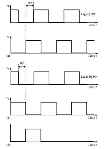
Pins for Channel A and Channel B give the quadrature signals shown in Figure a and b, and the Index pin gives the reference pulse signal shown in Figure c. Figure 2a shows the sensor outputs (v1 and v2) when the disk rotates in the clockwise (cw) direction; and Figure 2b shows the outputs when the disk rotates in the counterclockwise (ccw) direction. Several methods can be used to determine the direction of rotation using these two quadrature signals. For example,

1.      By phase angle between the two signals

2.      By clock counts to two adjacent rising edges of the two signals

3.      By checking for rising or falling edge of one signal when the other is at high

4.       For a high-to-low transition of one signal check the next transition of the other signal

Pulsed signal output of incremental encoder. (a) CW rotation; (b) CCW rotation; (c) Index pulse

Method 1: It is clear from Figure 2a and b that in the CW rotation, v1 lags v2 by a quarter of a cycle (i.e., a phase lag of 90°) and in the CCW rotation, v1 leads v2 by a quarter of a cycle. Hence, the direction of rotation may be obtained by determining the phase difference of the two output signals, using phase detecting circuitry.

Method 2: A rising edge of a pulse can be determined by comparing successive signal levels at fixed time periods (can be done in both hardware and software). Rising-edge time can be measured using pulse counts of a high-frequency clock. Suppose that the counting (timing) begins when the v1 signal begins to rise (i.e., when a rising edge is detected). Let n1 = number of clock cycles (time) up to the time when v2 begins to rise; and n2 = number of clock cycles up to the time when v1 begins to rise again. Ten, the following logic applies:

If n₁ > n₂ – n₁àCW rotation

If n₁ < n₂ – n₁àCCW rotation

Method 3: In this case, firstly high level logic of v₂ is detected and then check if v₁ is at rising or falling edge.

If v₁ is at rising edge when v₂ is at logic high à CW rotation

If v₁ is at falling edge when v₂ is at logic high à CCW rotation

Method 4: Detect a high to low transition in signal v₁.

If the next transition in signal v₂ is Low to High à CW rotation

If the next transition in signal v₂ is High to Low à CCW rotation